Simulation
Last updated: 2025-10-22
Checks: 7 0
Knit directory: qltan_postdoc_note/
This reproducible R Markdown analysis was created with workflowr (version 1.7.1). The Checks tab describes the reproducibility checks that were applied when the results were created. The Past versions tab lists the development history.
Great! Since the R Markdown file has been committed to the Git repository, you know the exact version of the code that produced these results.
Great job! The global environment was empty. Objects defined in the global environment can affect the analysis in your R Markdown file in unknown ways. For reproduciblity it’s best to always run the code in an empty environment.
The command set.seed(20250707) was run prior to running the code in the R Markdown file. Setting a seed ensures that any results that rely on randomness, e.g. subsampling or permutations, are reproducible.
Great job! Recording the operating system, R version, and package versions is critical for reproducibility.
Nice! There were no cached chunks for this analysis, so you can be confident that you successfully produced the results during this run.
Great job! Using relative paths to the files within your workflowr project makes it easier to run your code on other machines.
Great! You are using Git for version control. Tracking code development and connecting the code version to the results is critical for reproducibility.
The results in this page were generated with repository version 426f8e6. See the Past versions tab to see a history of the changes made to the R Markdown and HTML files.
Note that you need to be careful to ensure that all relevant files for the analysis have been committed to Git prior to generating the results (you can use wflow_publish or wflow_git_commit). workflowr only checks the R Markdown file, but you know if there are other scripts or data files that it depends on. Below is the status of the Git repository when the results were generated:
Ignored files:
    Ignored:    .Rhistory
Note that any generated files, e.g. HTML, png, CSS, etc., are not included in this status report because it is ok for generated content to have uncommitted changes.
These are the previous versions of the repository in which changes were made to the R Markdown (analysis/simulation.Rmd) and HTML (docs/simulation.html) files. If you’ve configured a remote Git repository (see ?wflow_git_remote), click on the hyperlinks in the table below to view the files as they were in that past version.
| File | Version | Author | Date | Message |
|---|---|---|---|---|
| html | d69197f | hmutanqilong | 2025-09-03 | Build site. |
| Rmd | c06385e | hmutanqilong | 2025-09-03 | Update_2025_09_02 |
| html | c06385e | hmutanqilong | 2025-09-03 | Update_2025_09_02 |
| html | a54969b | hmutanqilong | 2025-08-28 | Build site. |
| html | cbb6542 | hmutanqilong | 2025-08-28 | Build site. |
| Rmd | 2f4e8de | hmutanqilong | 2025-08-28 | Update_2025_08_28 |
Simulation: Exploring Categorical vs. Continuous Batch Covariate Adjustments in Negative Binomial Models
NB-GLM
We selected the negative binomial generalized linear model (NB-GLM) for analyzing simulated gene expression count data. Here are some brief rationales:
The linear regression model assumes a normal distribution of residuals, which count data violates, since gene counts are discrete and skewed. Moreover, linear model can predict negative count values, which don’t make sense. And for count data, the variance typically increases as the mean of counts increases.
The Poisson regression model is a good choice but requires equality between the mean and variance (\(Var(Y) = E(Y)\)).
The Negative binomial model:
In real world, the observed variance in count data is significantly larger than the mean, which called overdispersion. The NB-GLM can introduce a dispersion parameter (\(\alpha\)) to allow the variance to be greater than the mean.
\[ Var(Y)=\mu+\alpha\mu^2 \]
The dispersion parameter α is estimated from the data. If the data has no overdispersion, α will be estimated near zero, and the NB model effectively **converges to the Poisson model**. This makes it a flexible and safe choice.Simulation Scenarios:
- batch covariate without actual batch effects, meaning the batch variable simply represents sequencing groups without influencing the data.
- batch covariate with random batch effects, meaning it represents sequencing groups while simultaneously introducing unwanted and irregular systemic bias across different batches.
- batch covariate with linear batch effects and shuffled, meaning it represents sequencing groups while simultaneously introducing a linearly increasing systemic bias (e.g. simulating reagent loss or other technical drifts. as sequencing progresses). But this scenario can be easily adjusted by modeling batch as a numeric variable, so we further shuffled a proportion of cells across batches to generate a more complex batch structure.
Batch Variable Types in Model
- batch as categorical variable
- batch as numeric variable
- top 20 principle components (PCs) from non-targeting cells across batches
- top 20 sparse PLS-DA (Partial Least-Squares Discriminant Analysis) components from non-targeting cells across batches
- top 20 PCs from dummy batch matrix (bPC)
Notes: (The components derived from PLS-DA capture variance that is primarily driven by batch effects;
sPLS-DA is more effective and fast for high-dimensional expression matrix.)
Gene Expression Count Matrix
- No. of genes: 100
- proportion of differential genes: 0.1 (10 genes)
- No. of cells: 6000
- Prop. of targeting cells: 0.3 (1800 cells)
- No. of batches: 30
- Ratio of targeting and non-targeting cells in each batch: (60:140)
- No. of PCs / PLS / bPCs: 20
Evaluation index
- Type I error in null genes (excluding DE genes)
- Inflation factor, lambda
- Power check on DE genes
- FDR, TPR, Discovery Sig Genes
- FDR: after multiple correction, the proportion of false positive genes in all declared significant genes (TP + FP)
- TPR: the proportion of detected real DE genes in all real DE genes
- Discoveries: just number of significant DE genes.
- QQ plot of once simulation.
Batch effect demo
Boxplots of the expression counts for a gene across batches in simulation.
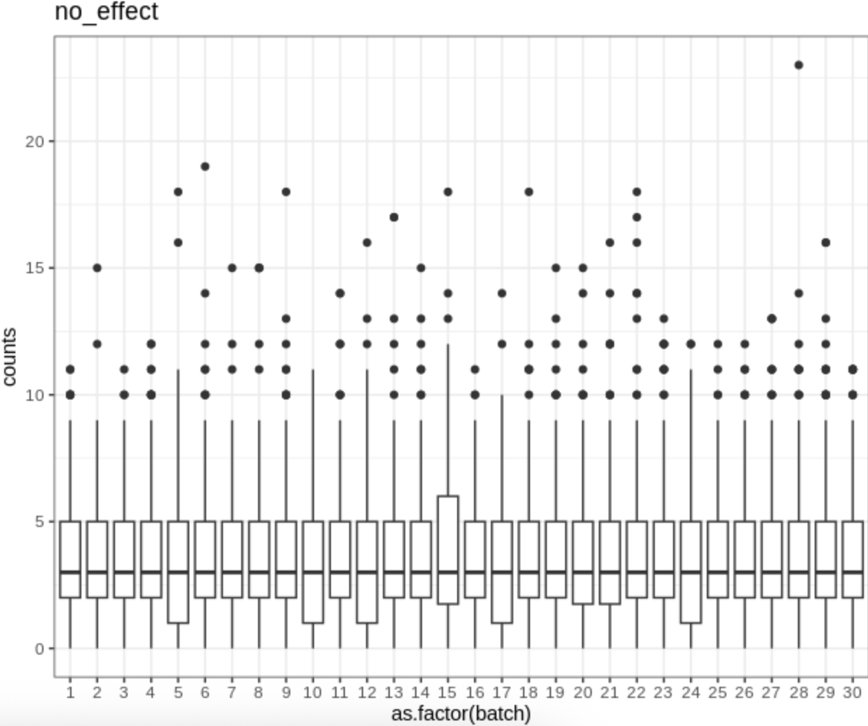
image.png
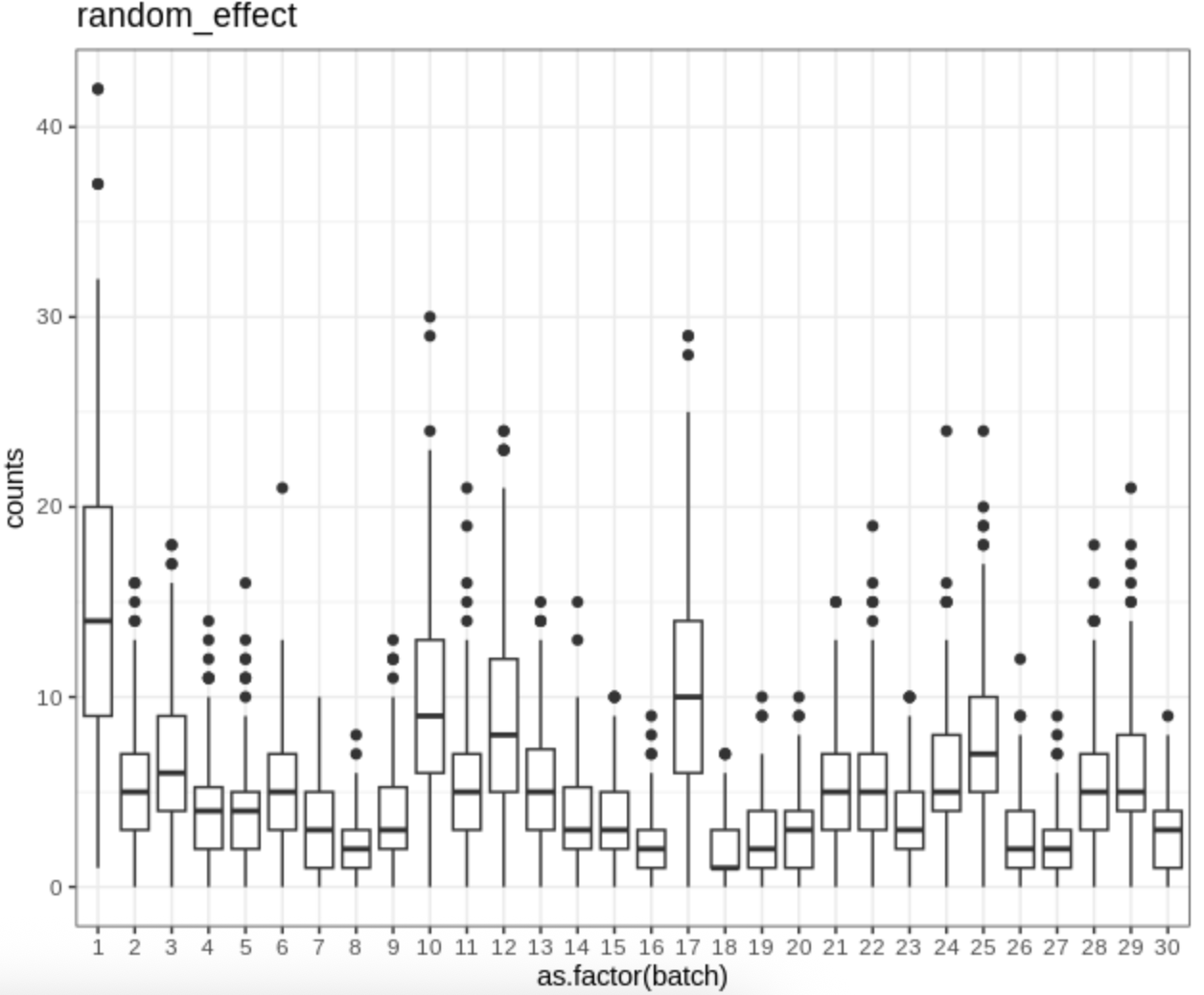
image.png
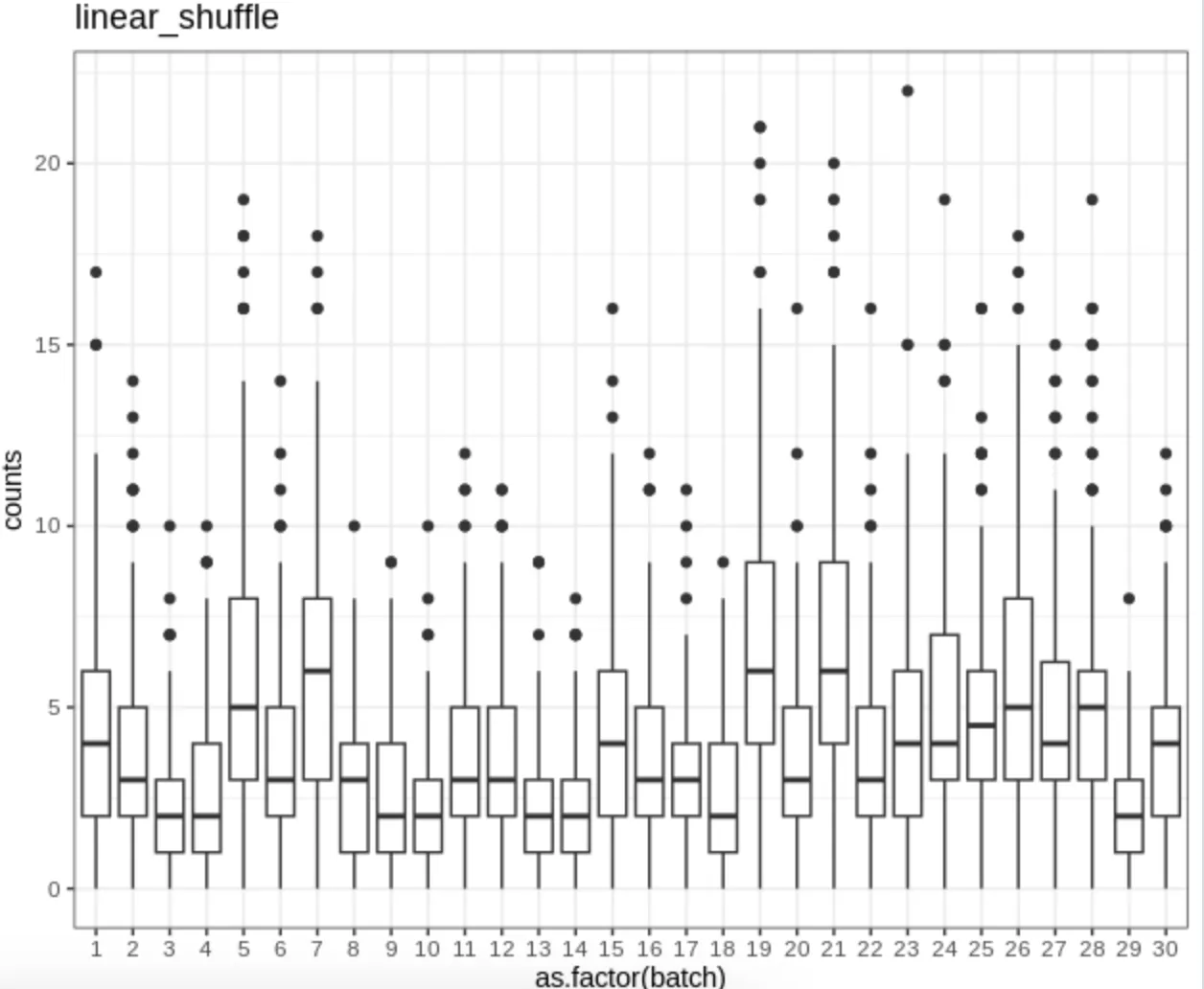
image.png
QQ plot of models including all types of batch covariates (once demo)
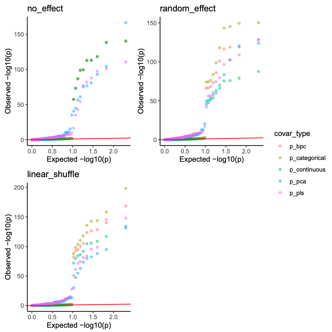
image.png
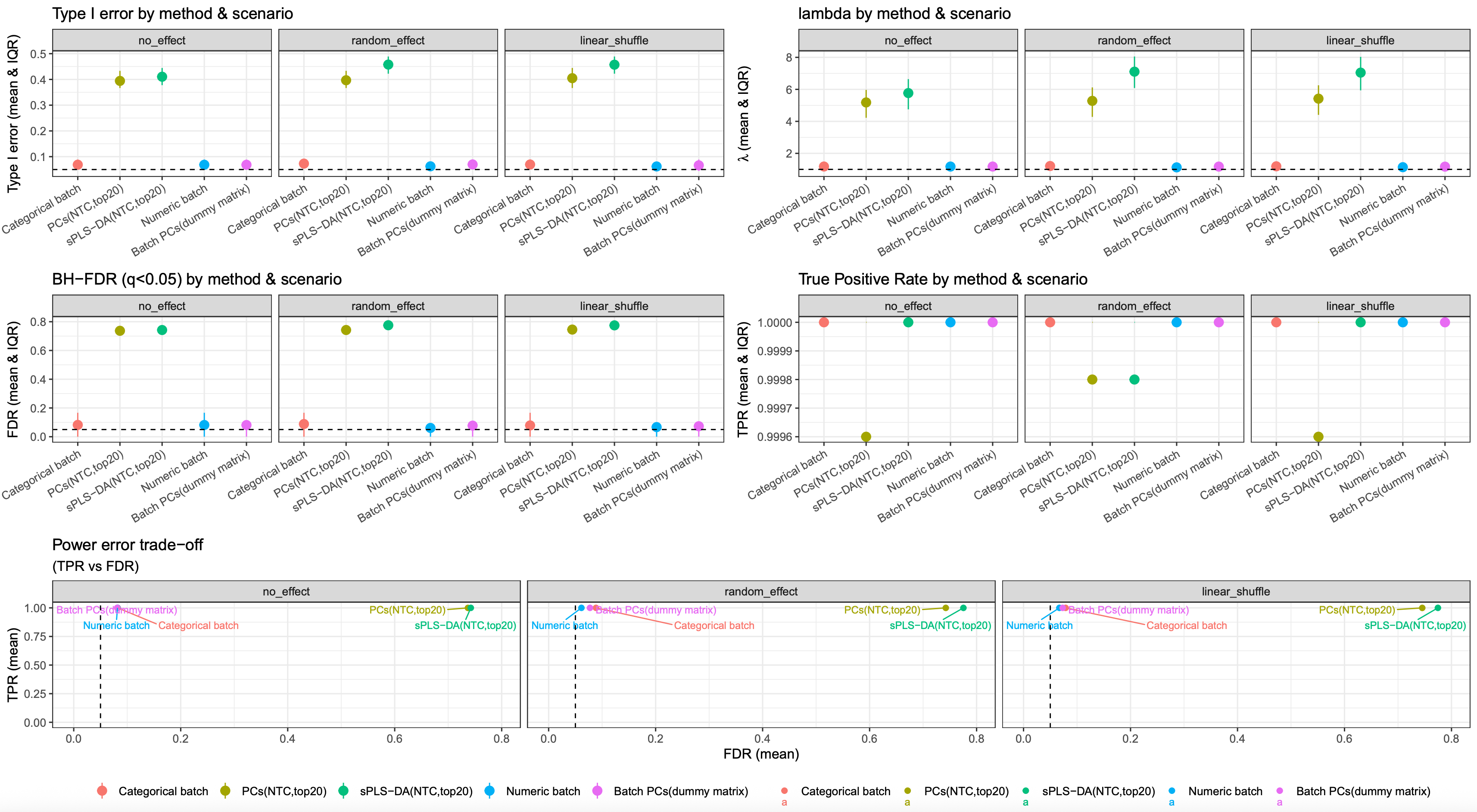
Replicate 500 times
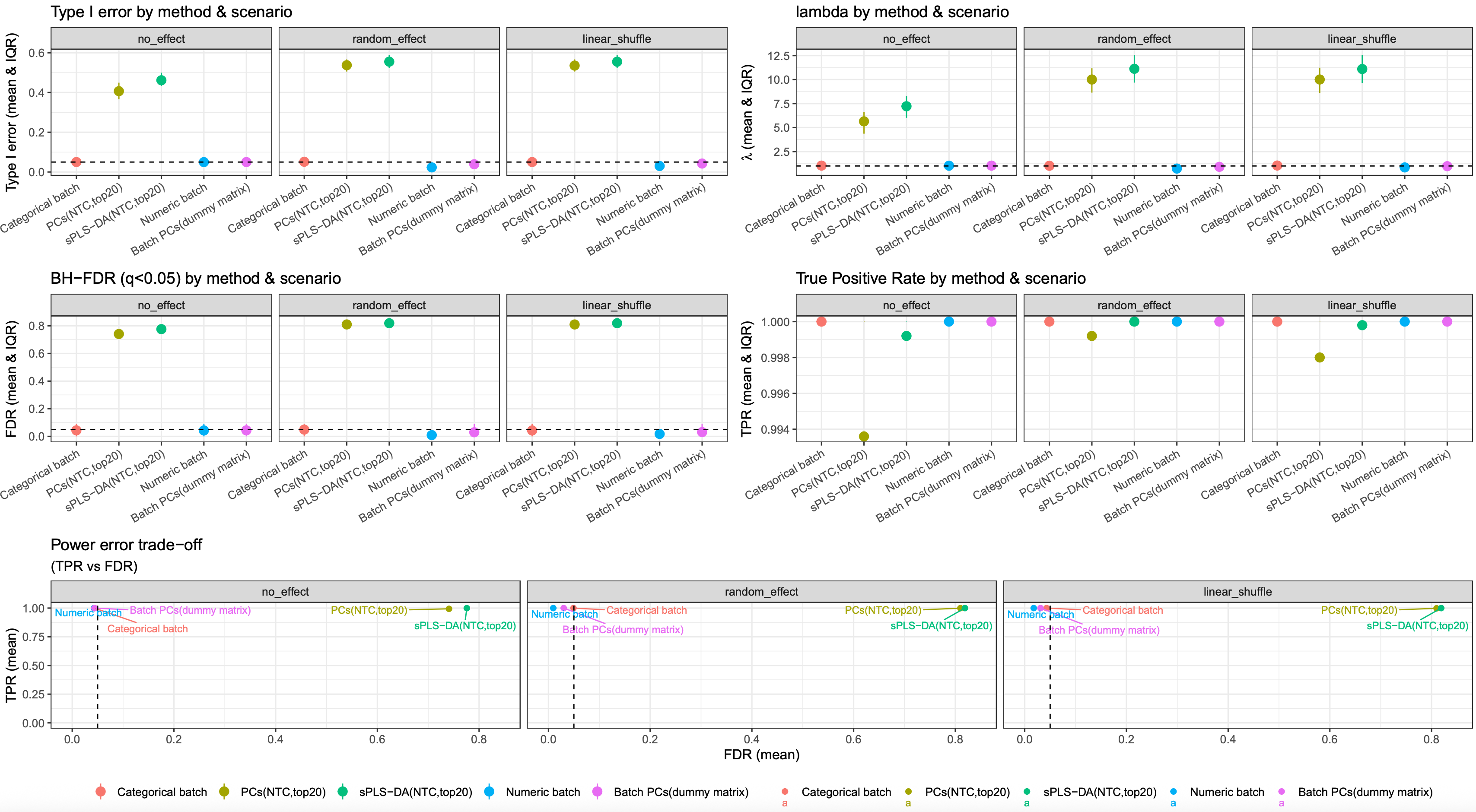
image.png
The 500 simulations indicate that representing batch as categorical, numeric, or via a dummy matrix based on batch PCs leads to similar results. Compared to other two results based on latent batch factor methods (PCA and PLS-DA), they all showed reduced type I error and FDR, with an almost 100% true positive rate (TPR)
Why? The logic seems reversed.
In above simulations, we assumed genes are independent with each other, and the batch and group variables are also orthometric, which makes batch variable as a “useless and harmless” variable, because we designed well for DE group. and PCA and PLS-DA maybe learned more useless information and overfit.
So we further simulated another three scenarios:
1. generate a count matrix with correlation among genes. In this count matrix, the correlation follows an AR(1) structure, meaning correlation decays exponentially with gene distance.
Here, we set rho 0.5, decay intensity sigma^2 0.4
Once simulation demo’s QQ plot: (some dots are overlapped)
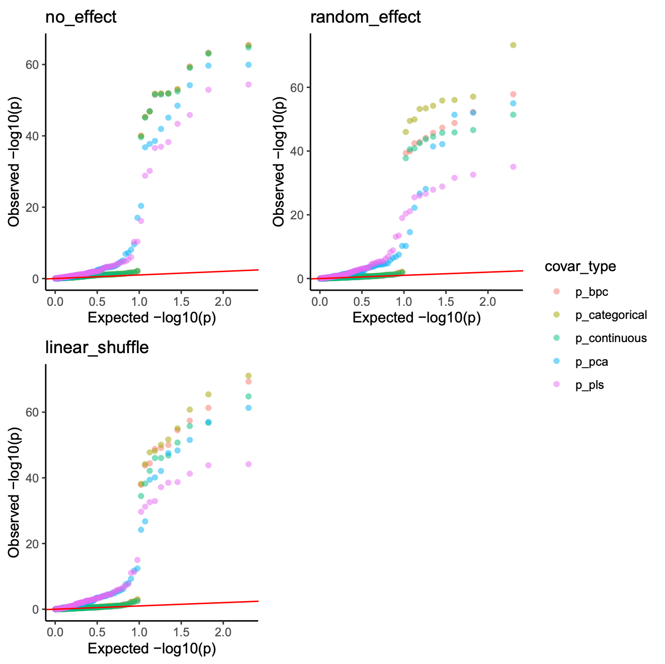
image.png
Simulation 500 times metrics results: (Type 1 error threshold is 0.05; FDR threshold is 0.05)
Type 1 error threshold is 0.05; FDR threshold is 0.05
Type 1 error threshold is 0.05; FDR threshold is 0.05
2. based on gene correlation structure, we further simulated a kind of unbalanced experiment design, i.e. proportions of cases and controls varied across batches.
In some batches, only ~5 cases were included. Under this setting, batch and group membership became correlated.
Once simulation demo’s QQ plot: (some dots are overlapped)
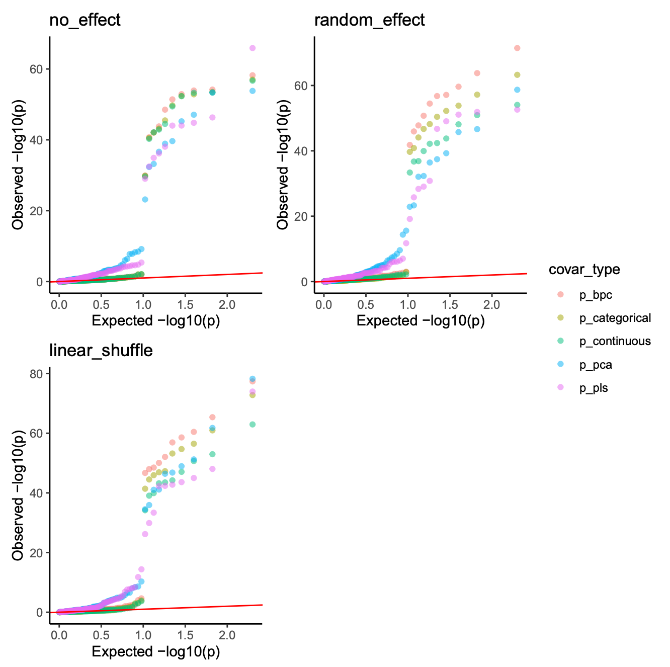
image.png
Simulation 500 times metrics results: (Type 1 error threshold is 0.05; FDR threshold is 0.05)
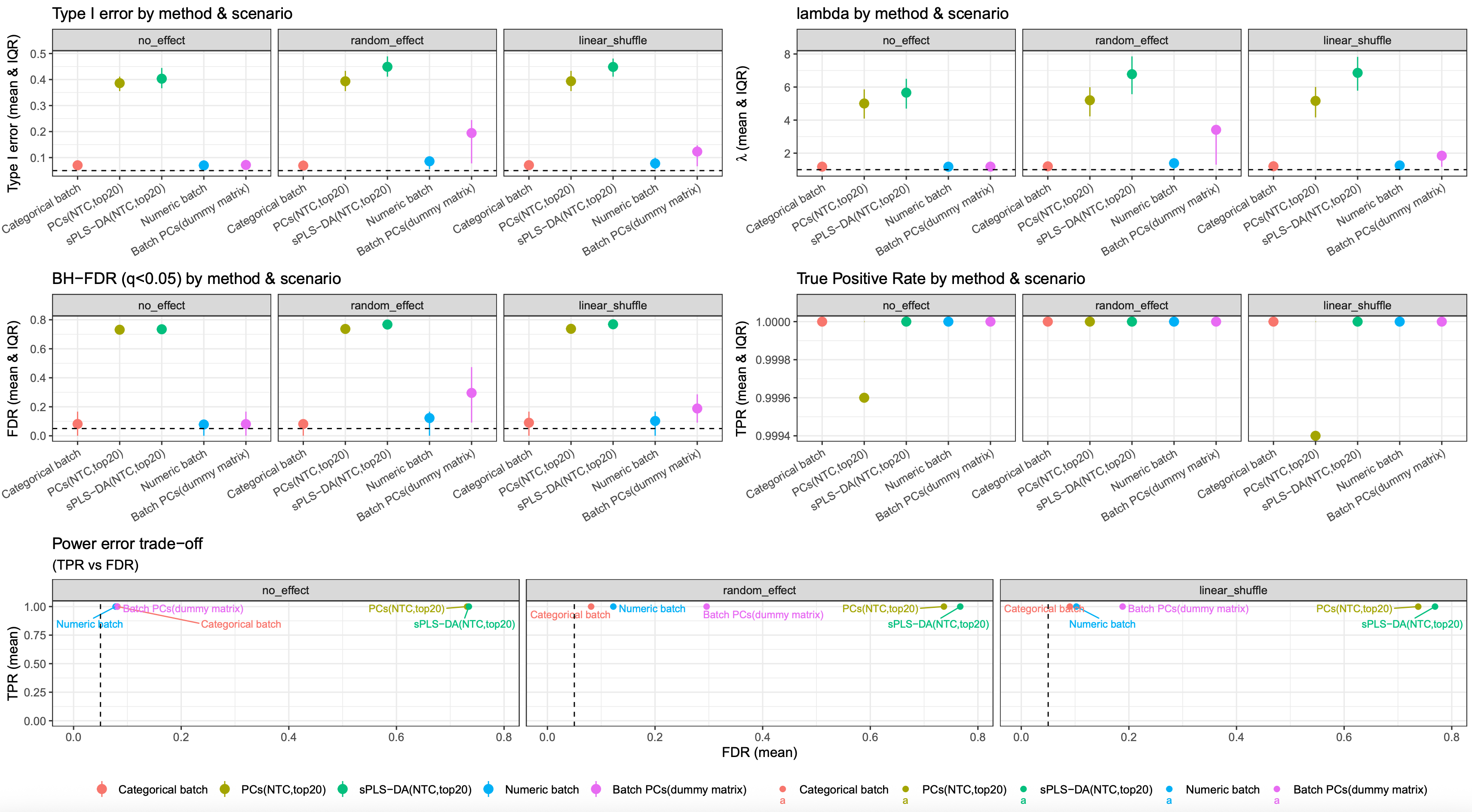
image.png
In this case, every method has a higher type I error and FDR, but batch as categorical and continuous is still robust.
3. Still based on the same gene correlation structure described above, we generated another type of count matrix. In this setting, a subset of genes was correlated with the batch variable, meaning that the batch effects on the same gene expression differed across batches. Statistically, this was implemented by simulating a random intercept for batch effects.
Once simulation demo’s QQ plot: (some dots are overlapped)
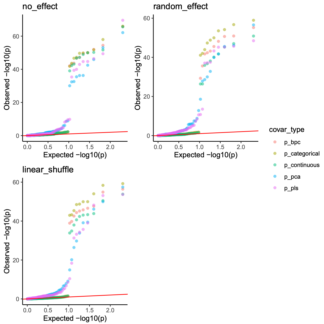
image.png
Simulation 500 times metrics results: (Type 1 error threshold is 0.05; FDR threshold is 0.05)
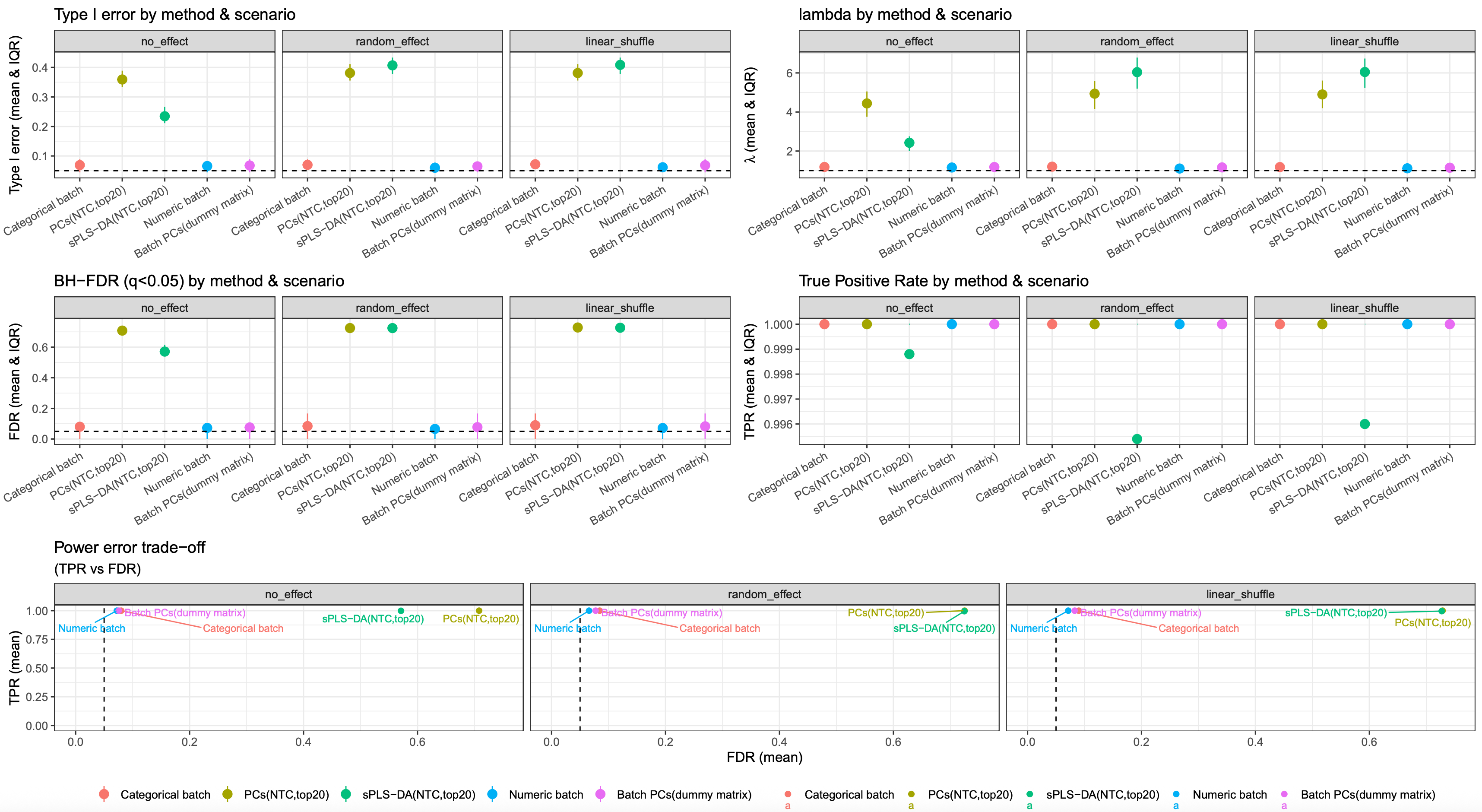
image.png
Conclusion
if a dataset dose not suffer from a severe flaws in experiment design, batch effects can be adjusted by modeling batch as categorical, continuous, or through PCs derived from a dummy batch matrix.
Patch
I noticed all batch number are treated as being equally spaced when modeled as a continuous covariate. In this scenario, batch dummy design matrix will be more competitive and precise.
In this simulation, I will assign different batch numbers and evaluate scenarios including no batch effects, random batch effects, linear batch effects with partially shuffled cells.
- The original batch number is 1, 2, 3, 4, 5, 6, …, 28, 29, 30
- The new batch number is like 4, 10, 14, 15, 21, 22, 27, 29, 39, 43, 44, 46, 47, 49, 52, 54, 56, 57, 60, 64, 65, 69, 75, 80, 83, 85, 86, 93, 94.
Once simulation demo’s QQ plot:
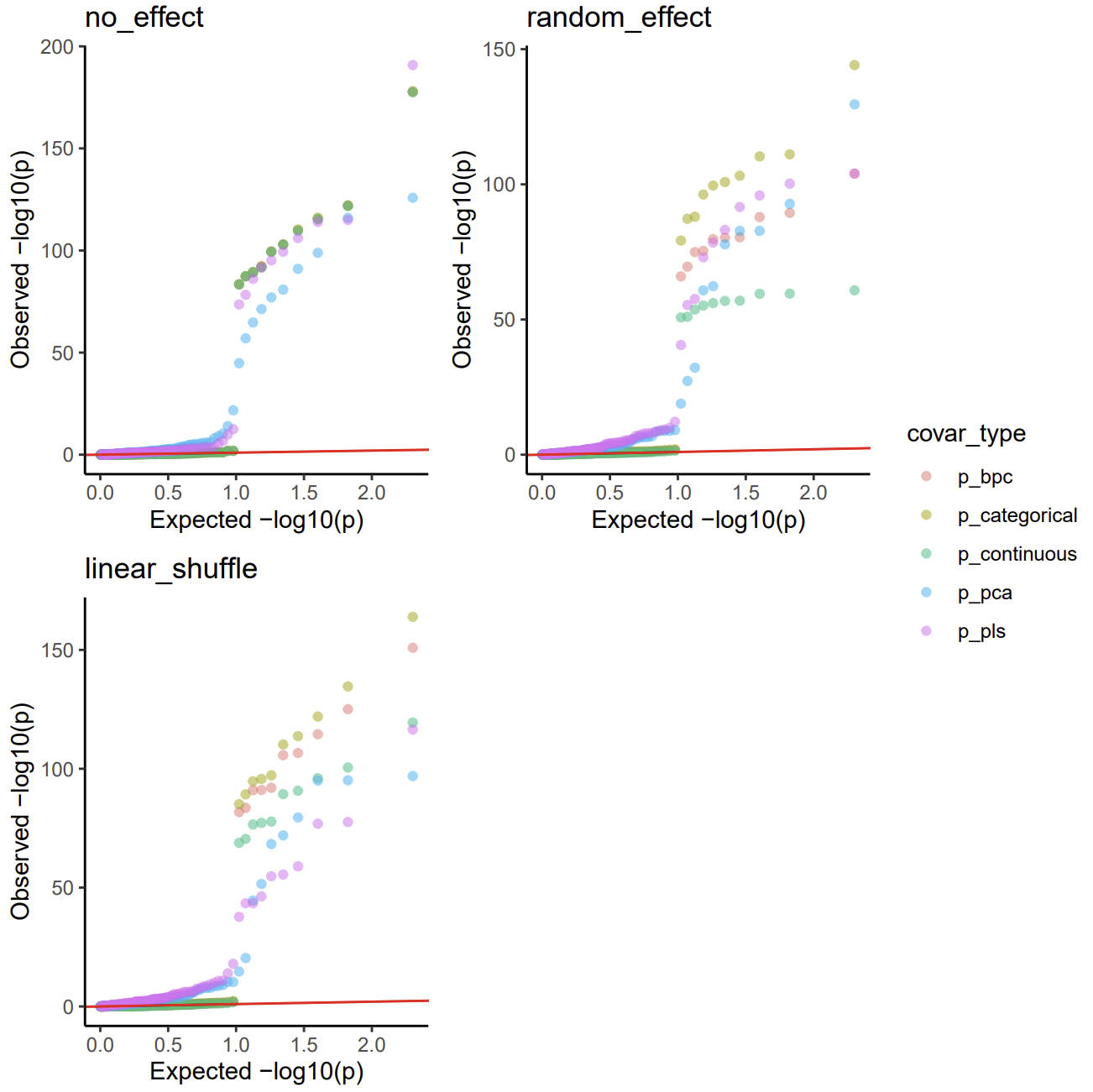
image.png
Simulation 500 times metrics results: (Type 1 error threshold is 0.05; FDR threshold is 0.05)
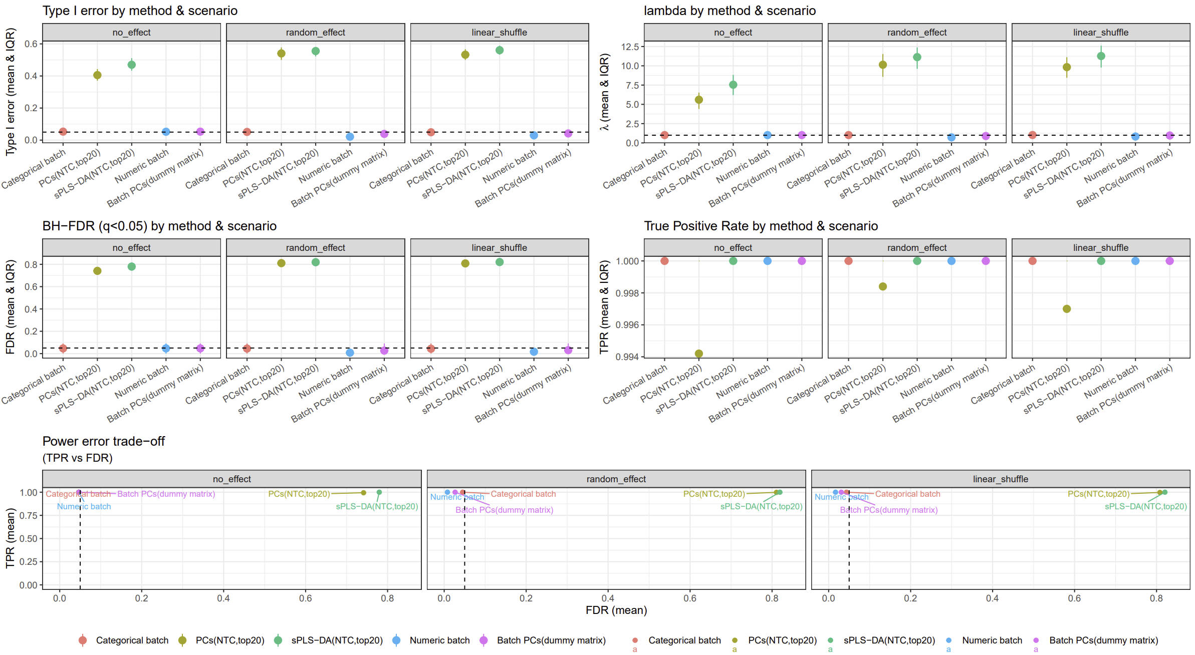
image.png
from this simulation result, modelling batch variable using continuous variable or PCs derived from batch dummy matrix is still a robust strategy.
sessionInfo()R version 4.1.0 (2021-05-18)
Platform: x86_64-pc-linux-gnu (64-bit)
Running under: CentOS Linux 8
Matrix products: default
BLAS/LAPACK: /software/openblas-0.3.13-el8-x86_64/lib/libopenblas_skylakexp-r0.3.13.so
locale:
[1] LC_CTYPE=en_US.UTF-8 LC_NUMERIC=C
[3] LC_TIME=en_US.UTF-8 LC_COLLATE=en_US.UTF-8
[5] LC_MONETARY=en_US.UTF-8 LC_MESSAGES=en_US.UTF-8
[7] LC_PAPER=en_US.UTF-8 LC_NAME=C
[9] LC_ADDRESS=C LC_TELEPHONE=C
[11] LC_MEASUREMENT=en_US.UTF-8 LC_IDENTIFICATION=C
attached base packages:
[1] stats graphics grDevices utils datasets methods base
other attached packages:
[1] workflowr_1.7.1
loaded via a namespace (and not attached):
[1] Rcpp_1.0.12 compiler_4.1.0 pillar_1.10.2 bslib_0.7.0
[5] later_1.2.0 git2r_0.32.0 jquerylib_0.1.4 tools_4.1.0
[9] getPass_0.2-2 digest_0.6.33 jsonlite_1.8.7 evaluate_0.23
[13] lifecycle_1.0.4 tibble_3.2.1 pkgconfig_2.0.3 rlang_1.1.6
[17] cli_3.6.1 rstudioapi_0.15.0 yaml_2.2.1 xfun_0.45
[21] fastmap_1.1.1 httr_1.4.2 stringr_1.5.1 knitr_1.48
[25] fs_1.6.3 vctrs_0.6.4 sass_0.4.9 rprojroot_2.0.4
[29] glue_1.6.2 R6_2.5.1 processx_3.8.4 rmarkdown_2.27
[33] callr_3.7.6 magrittr_2.0.3 whisker_0.4.1 ps_1.7.5
[37] promises_1.2.0.1 htmltools_0.5.8.1 httpuv_1.6.1 stringi_1.6.2
[41] cachem_1.0.8